Detect Rhythm Episodes
DataView contains facilities to help detect and mark periods of rhythmic or oscillatory activity embedded in aperiodic data. The input to these facilities is either the raw waveform data themselves, or events that have been extracted from the data.
Algorithm
The key defining feature that makes something rhythmic is the regularity of occurrence of particular activity motifs. If these repeat at more-or-less fixed intervals, that activity is rhythmic. If the motifs occurs at random intervals, the activity is arrhythmic. This is, of course, not a binary distinction, and exactly how regular the activity has to be before it is considered rhythmic is a matter of judgement.
For raw waveforms, regularity is detected by looking for a trough followed by a peak in the autocorrelation of the waveform. For events, regularity is detected by looking for a contiguous series of events with a low coefficient of variation in the intervals between them.
Detecting Rhythms in Waveforms
Note that this algorithm works best if you already know that your data contains some rhythmic activity through visual inspection, and you want an objective way of detecting all such activity within the recording.
- Load the file fly buzz.
This shows a segment of an audio recording of fly courtship song. There are silent periods, and then periods where the fly emits a buzzing sound. The display shows a transition from non-buzzing to buzzing. We want to detect the buzzes. (Note: the file is actually a montage from which some data have been eliminated.)
Quick Start Steps
- Find a region where there is rhythmic activity in the recording, and put it in the approximate middle of the main view (the sample file loads with an appropriate region displayed).
- Select Event edit: Rhythm in data to open the Trace autocorrelation rhythm detect dialog.
This dialog is non-modal, so you can switch away from it and perform other other analyses if you wish.
Note that for this sample file, the default values are all appropriate for the analysis, so you could just click the Analyse button. - Select the correct Data trace for analysis and Event channel for results storage.
- Click the Sync button to preview rhythmic data in the upper data display
- Click the Expand (< >) or Contract (> <) buttons until the Rhythm limits: Max has a value that is somewhat greater than the largest cycle period of the rhythm of interest. This sets the lag for the calculation of correlation coefficients. The visual cues in the dialog display help get a suitable value (see next point).
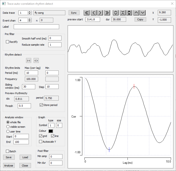
- At this point you should see clear peaks and troughs in the lower correlation display in the dialog, and several cycles of the rhythm should be visible in the upper data display. The screenshot below shows this situation.
- Click Analyse, and observe the events in the main view.
- Adjust parameters if necessary according to the detailed description below
Details
The analysis works by taking a chunk of data of length set by the Sliding window parameter, and calculating the autocorrelation coefficients at lags up to the defined Maximum period. It then searches forward through the coefficients to find the first trough followed by a peak in the coefficient values. If the trough-to-peak height is above the Threshold value, then the window is considered to contain rhythmic activity. It then advances to the next chunk by the defined Step and repeats the analysis. The step would normally be shorter than the sliding window, so that analysis regions overlap. Rhythmic regions are marked by events in the selected channel.
Note: autocorrelation coefficients are insensitive to the amplitude of the source data within the analysis window, so the Threshold refers to the degree of rhythmicity, not the size of the raw signal (see Post filter below if that is a matter that needs consideration) .
The two graphs in the dialog show a preview of the analysis. The upper graph shows a Sliding window length of the raw data that is being analysed, the lower graph shows the correlation coefficients for that window.
There are 4 key parameters for rhythm detection.
- Rhythm limits: Period: Max (corr lag): This sets the lag over which correlation coefficients are calculated. It should have a value somewhat larger than the longest expected period in the rhythm of interest, hence the name in the dialog box.
- Sliding Window: This sets the window over which the analysis is performed. It should be long enough to contain at least 2 complete cycles of the rhythm. A longer window improves detection, but at the expense of time resolution. The default value is 3 times the lag.
- Step: This sets the time by which the sliding window is advanced for each step during analysis. The smaller this value the more fine-grained the time resolution, but the slower the analysis.
- Threshold: A trough followed by a peak in the correlation values is an indication of rhythmicity, and the normalized trough-to-peak height is shown as the rhythmicity index. The index indicates the regularity of the rhythm within the sliding window currently being analysed, and if the index exceeds the threshold value, then that section of data is regarded as rhythmic. The default threshold value is 0.5, but this may need to be adjusted according to the characteristics of the data.
Note that any trough or peak will be counted, so if the autocorrelation graph is a bit jagged, the algorithm can fail. This can usually be fixed by using the Smoothing pre-filter.
The key parameters can be adjusted using the interactive preview displayed in the two graphs of the dialog box. The location of the preview data within the main recording can be set by editing the preview start time explicitly, or by using the navigation buttons above the graph. A quick way to get the preview in the right location is to centre a section of rhythmic activity in the main view, and then click the Sync button, which makes the data preview start at the main screen centre. The sample data file is already correctly positioned, so you can click Sync immediately.
- Click the Left page navigation button (
 ) in the dialog.
This moves the preview one sliding window earlier in the file, and we can see that the data display is now half occupied by non-rhythmic data, and there is a corresponding reduction in the Rhythmicity index.
- Click Left page again.
The coefficient preview still shows peaks and troughs, but these are rather chaotic, and much smaller. The preview window shows that data in this region do have some rhythmicity (probably microphonics), but it is lower amplitude and higher frequency than the main song rhythm. The rhythmicity index is well below the default Threshold value, so it would not be scored as rhythmic in analysis.
- Click the Right page navigation button (
 ) twice to return to the highly rhythmic data.
The first 3 key parameters can be doubled and halved simultaneously using the Compress (><) and Expand (<>) buttons respectively. If the lag value is edited directly, then the Sliding window and Step parameters change automatically to be 3 times and 1 times the lag value respectively. This is because this is a reasonable default setting. However, the Sliding window and Step can be set independently of the lag if desired.
Note that because autocorrelation essentially works in the frequency domain, the timing precision with which the onset and offset of rhythms is detected is limited by the size of the Sliding window. Longer windows allow the detection of weaker rhythms contaminated by noise, but at the expense of loss of precision in timing. This loss can be partly offset by setting the Step value so that the Sliding windows overlap, as is the case with the default settings.
- Click the Expand button (
 ) and note that the rhythmicity index value disappears. This is because we have set the lag to a value shorter than the rhythm period, so no peak is visible following the trough in the correlation preview, and no rhythm is detected.
 - Now click the Compress button (
 ) twice, and observe that multiple troughs and peaks are visible in the correlation preview. This is suboptimal, so click the Expand button to return to the starting parameters.
 - Click Analyse.
- Click the Show all button (
 ) in the main Chart view toolbar to see the results:
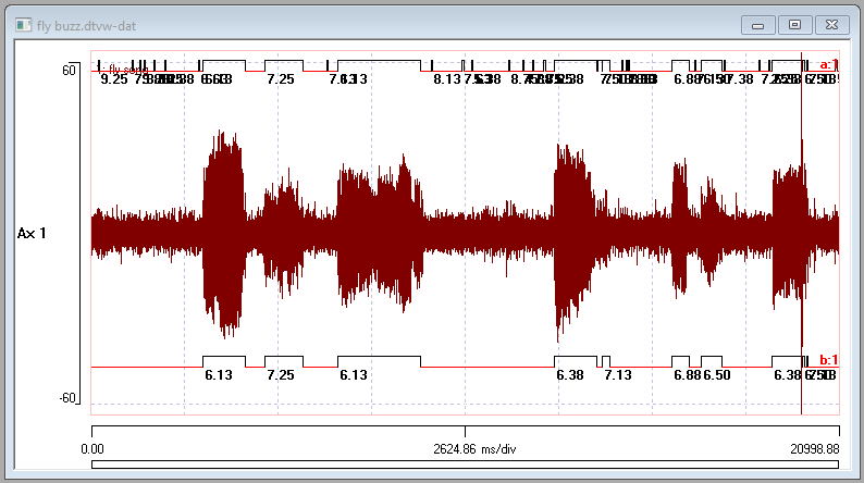
Event channel a shows the output of the analysis. The main episodes of fly song have clearly been detected, but there are also quite a few brief events which appear to delimit signals within the noise (e.g. the first few events). However, detailed examination of these shows that there is indeed apparent rhythmic activity in the data, but this is brief and low amplitude. The autocorrelation algorithm is amplitude insensitive, and so these episodes are detected along with the lengthier and higher-amplitude episodes which are the ones we are interested in. We can improve things by applying a post-filter to the events.
Post-Filter
- Select the Analyse: Measure data: Measure box command from the main menu, and draw a box in the main view around the data trace in the first part of the recording, where there are brief events with no obvious high-amplitude activity.
- Note that the trace 1 peak-to-peak amplitude in this region is about 20.
- Close the Results dialog.
- Go back to the Rhythm detect dialog, and enter 25 into the Min amp box in the Post filter group near the bottom of the dialog.
Note that you could also set a minimum duration if you wished, but you can leave that at 0 for now. - Set the event channel to b.
- Click Analyse.
Now only events in which the data trace peak-to-peak amplitude exceeds 25 are retained. These are shown in event channel b (at the bottom of the view in the figure below).
Pre-Filter: extracellular recording
The Trace auto-correlation rhythm detect facility contains pre-filtering options that allow you to rectify and smooth the signal before analysing it, which would be appropriate for an extracellular recording. However, the Transform: De-mean/median, rectify, smooth menu command give more flexibility, and is recommended as an alternative pre-processing step.
Spectral analysis
The numerical value associated with each event detected by this method shows the average period (ms) of the rhythm during the event. The second buzz episode has a slightly longer period than the first (7.25 vs 6.13 ms) as well as having a lower amplitude.
- If you have sound enabled on your computer, select the Sound: Play menu command.
You should hear that the second buzz is slightly lower in pitch than the first, as well as being softer. You should also hear that there is variation in the pitch (frequency) within the buzz episodes, so be aware that the event numerical value is just a guide to the average value of the period.
You can examine the frequency characteristics of the buzz episodes in more detail with spectral analysis. Full details of the various options are given here, but the following instructions "cut to the chase".
- Select the Analyse: Spectrogram menu command to open the Spectrogram dialog.
- Set the Number of time bins to 80.
- Set the Frequency resolution: Bins to 512.
- Set the display scale Upper Hz to 500.
- Click the Spectrum button to open the Spectral results dialog in parallel with the Spectrogram.
- Uncheck the Autoscale X box.
- Set the right-hand frequency scale to 500 Hz.
- In the main Spectrogram dialog, drag the slider box (between the coloured map of spectral density and the chart view of the data) to align with the highest power (dark red colour) in the first buzz episode in the density map.
- In the Spectral results dialog hover the mouse over the prominent peak, and note the Frequency read-out, which should be about 160 Hz.
- Scroll down the text list at the top of the dialog, and note that the highest power occurs at bin 21, which is 164.06 Hz. This corresponds to a period of 6.1 ms, which fits with the numerical value of the event marking this episode.
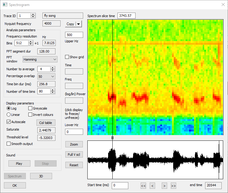
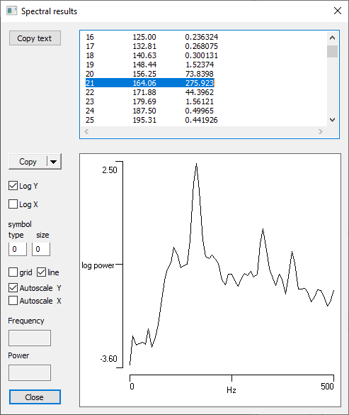
- In the main Spectrogram dialog, drag the slider box to the second buzz episode and note that the peak in the Sectral results shifts slightly to the left, corresponding to the slightly lower frequency of this episode.
- When you are done admiring the various analyses, Close any dialog boxes you have open.
Detecting Rhythms in Events
DataView can also look for rhythms within event trains without reference to the waveform data. Bouts of rhythmic activity are identified as regions in which the interval between events has a low coefficient of variationThe coefficient of variation is simply the standard deviation divided by the mean. (CV), i.e. the interval does not vary much.
- Close and re-load the file fly buzz to get back to the default display before analysis.
- If it is already open, delete any event channels from the previous analysis.
- Select Event edit: Threshold menu command to open the Threshold dialog.
- With the default Threshold source: user value selected, set the On: +ve value to 0 to detect zero-crossings as events.
The dialog preview should now look like this:
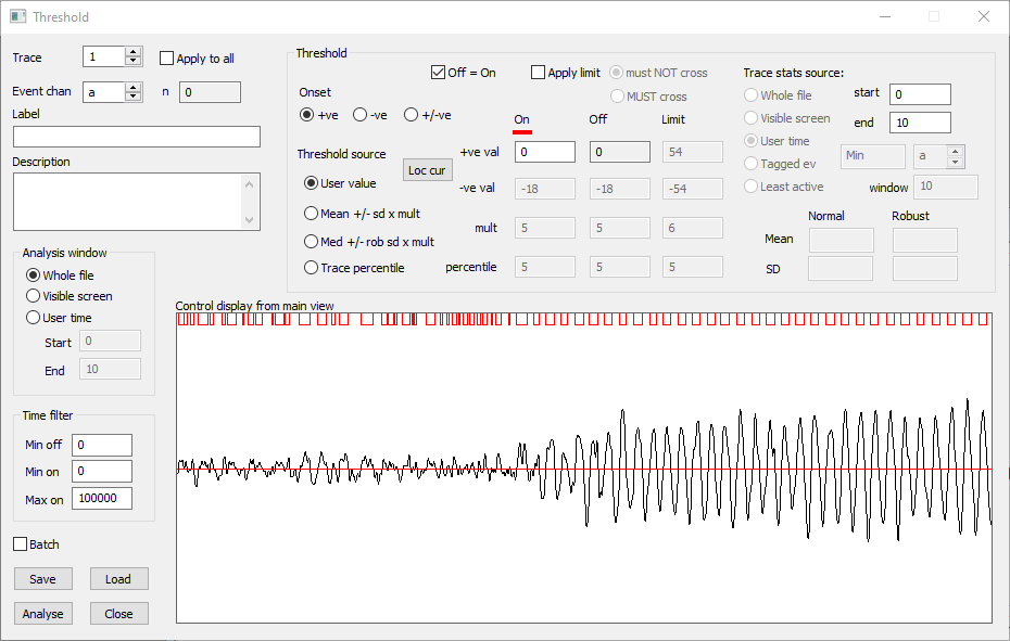
The events within the buzz section of data are regularly spaced, reflecting the regular oscillations of the waveform. The events within the noise data are much less regular.
- Click Analyse to write the events to the main file, and Close the Threshold dialog.
- Select the Event edit: Rhythm in events menu command to activate the Rhythm detect dialog box. This is non-modal, so you can switch between it and the main display.
The dialog box should now look like the image below.
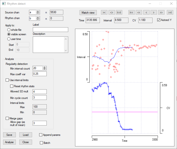
The Minimum interval count specifies the minimum number of consecutive regularly-spaced intervals that will be counted as a rhythm. The default value is 20, but if you know that the episodes of rhythmic activity that you are looking have fewer cycles than this, you can reduce this value. The minimum count is just 2 (i.e. three events with just 2 intervals between them). However, be aware that the chance of detecting spurious rhythms in random data is very high when a “rhythm” is defined with such a short episode length.
The algorithm starts at the beginning of the specified analysis region (which by default is the visible screen) and takes a series of consecutive intervals between events, with the number set by the Minimum interval count parameter. It calculates the mean and standard deviation of the intervals in this series, and hence the coefficient of variation. It then advances by one event, and repeats the calculation. This continues through the specified analysis region. Data are regarded as rhythmic when the CV drops below a threshold set as the maximum coefficient of variation (Max coeff var: there is a draggable horizontal cursor in the CV graph which interacts with this value).
There are two graphs in the dialog box, both initially displaying data derived from the section of data visible in the main display. The upper graph shows the raw intervals between events (red dots) and the running mean of the intervals over the Minimum interval count series (blue line). The lower graph shows the CV of the event series starting at the time given by the X axis. It is clear that as the data make the transition from baseline noise to the buzz, the intervals become regular and the CV drops to a low value.
The reason that the CV and running mean lines stop before the right-hand end of the graph is that their time values are registered to the start of the interval series, which by default is 20 intervals long. So their values terminate 20 intervals before the interval values themselves.
- Set the Minimum interval count to 5.
Now two episodes of rhythm are detected (i.e. the CV graph drops below threshold twice).
- Click Analyse to write the detected rhythm to the data in the selected Rhythm channel (b in this example)
Examination of the data in the main view shows that the first episode is in fact generated by a period in which the random noise in the signal just happens to produce a series of events with fairly regular intervals. This illustrates an important point about the algorithm: it is scale invariant. The spurious rhythm has much higher frequency than the real rhythm, but is still detected due to the definition of a rhythm as a period of events with regular intervals between them. Similarly, since the algorithm is working with events, it has no knowledge of the amplitude of the signal generating the events. There are many filtering options within DataView that could eliminate the spurious rhythm, but the easiest is to return to a longer sliding window.
- Reset the Minimum interval count to 20.
- Check the whole file option within the Apply to group.
- Click the Analyse button.
- Click the Show all toolbar button (
 ) in the main Chart view.
 - Click the Match view button in the dialog to make the interval and CV graphs show all the data.
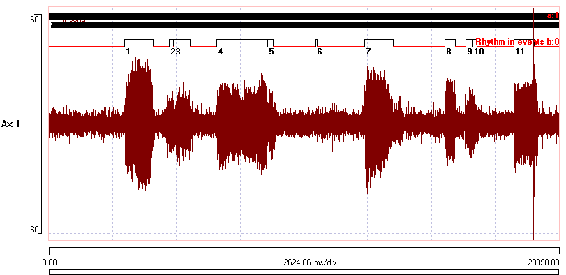
The main view should now look like this:
Post filter
There are two "issues" with the events in channel b: false negative and false positive episode detection.
False negative
The first issue is evident in the occurrence of occasional "drop-outs", where what looks like a single episode of buzzing has been detected as two events (e.g. events 9 and 10). If you zoom in on these using the Horizontal magnify button (![]() ) in the main toolbar you will see that they mainly caused by "jitter" in the initial event-detection routine where the waveform crosses the 0 level more than once within a cycle. This briefly elevates the CV and disrupts the event rhythm. These can be dealt with as follows:
) in the main toolbar you will see that they mainly caused by "jitter" in the initial event-detection routine where the waveform crosses the 0 level more than once within a cycle. This briefly elevates the CV and disrupts the event rhythm. These can be dealt with as follows:
- Check the Merge gaps box in the Rhythm detect dialog.
- Set the Rhythm channel to c to write events into a new channel.
- Click Analyse again.
Now the search algorithm makes a second pass through the data and merges any pair of episodes that are separated by a gap that is less than a specified multiple of the mean of the interval of the first episode. With the default multiplier of 3, events 4+5 and 9+10 in channel b are merged, but there is still a gap between events 2 and 3 because the period of jitter is more extended.
- Increase the multiplier from 3 to 8.
- Click Analyse again.
Now each buzz episode is marked by a single event, which was the desired outcome.
Note: An alternative approach would be to apply a moving average smoothing filter to the raw waveform before using the event Threshold detection method, thus reducing the jitter at source, . This can reduce episode disruption caused by jitter, but can increase the second of the two issues mentioned above - false positive detection.
False positive
The second issue is evident in event 6 in channel b (event 4 in the new channel c). Here, a section of noise happens to just meet the criteria for rhythmicity, and has been marked as such. The algorithm is behaving correctly, but the low amplitude of the signal encompassed by the event suggests that it is not a real buzz episode.
Since the problem involves the actual data rather than the event timing, we have to use facilities outside the Rhythm detect dialog, since this only deals with events.
We can deal with this as follows:
- Select the Analyse: Measure data: Measure box menu command and drag a box around a section of data that is clearly noise (the section between the recording start and the first vertical grid line in the chart view would be suitable).
- The Results dialog shows that the peak-to-peak amplitude in Trace 1 in this section (i.e. the noise section) is about 20.
- Close the Results dialog.
- Select the Event edit: Filter: Value filter menu command to open the Value filter dialog.
- Set the Source event channel to c.
Note that the default Destination channel is d, which should currently be empty. - Set the Trace to 1. This is essential, since we need to measure values from the data trace.
- The default Filter factor pre-selected from the drop-down list is P2P amp (peak-to-peak amplitude), which is what we want.
- Set the Min val to 25, which is a bit larger than the noise peak-to-peak amplitude.
- Click Apply, and look at the main view to check that the brief event (4 in channel c) has been eliminated in channel d, while all the other events have propagated through unchanged.
- Close all the dialogs that are currently open.
You now have a series of events in channel d marking each buzz episode within the file.
List Rhythmicity/Period
You can get a list of the rhythmicity index and average period for each buzz episode.
Note: This is independent of any of the preceding analyses - you can use the following procedure even if you simply marked the buzz episodes manually.
- Select the Event analyse: List/save event parameters menu command to open the Event Parameter List dialog.
- Set Event channel 1 to d (or whatever channel marks your rhymic episodes).
- Set the Parent to 1 (or whatever trace contains the source waveforms).
- Check the ID box in the Event-specific parameters group.
- Check the Autocorr rhythm info box in the Data value parameters group.
- Click List.
The Results dialog will display a list of the Event Id, on-time, rhythmicity index, and the average rhythm period for each event. The values are calculated "behind the scenes" from a statistical autocorrelation (normalized autocovariance) analysis of the waveforms within each event.
You could measure these values explicitly for a single episode thus:
- Set the main view start time to 3100 and the end time to 4300 ms (giving a timebase of 150 ms/div).
- Select the Analyse: Auto-correlation menu command to open the Trace auto-correlation dialog.
- Set the Analysis window to the visible screen - the default values of the other parameters are suitable.
The rhythmicity index is the trough-to-peak amplitude from the first trough in the covariance graph (marked with a red tick) to the second peak (marked with a blue tick), and the period is the lag to the second peak. The index (idx) and period are reported in the Rhythmicity section of the Correlation group of the dialog.